|
If you live in the Bay Area, you may have noticed the smoky haze that covered San Francisco and the surrounding areas earlier this month. Caused by several large wildfires in the Sonoma County, it greatly reduced air quality and visibility, and made me, and many others, reluctant to go outside. You may have also heard in the news about the devastation of Santa Rosa (where the fire destroyed 3,000 homes causing $1.2 billion in damages) along with other communities in the Sonoma County. All the while, the cause of the string of wildfires is still unknown and under investigation. Problem Overview These recent events was my motivation for my third project at Metis, Project McNulty. For this project I aim to create a classification model to predict the cause of a wildfire given its features, and create a tool in the form of a Flask application that could help authorities determine the cause of a fire when reasons are unknown. This application would also be able to determine the highest probable cause of wildfires in a given location to help decision-makers take steps to mitigate the risk. The data I used for this project is a Kaggle dataset and it consists a spatial database of 1.88 million wildfire events that occurred in the United States from 1992 to 2015 and was generated to support the national Fire Program Analysis (FPA) system. Some of the information given for each fire event included the location, the discovery date, the cause, the size, and the containment date. 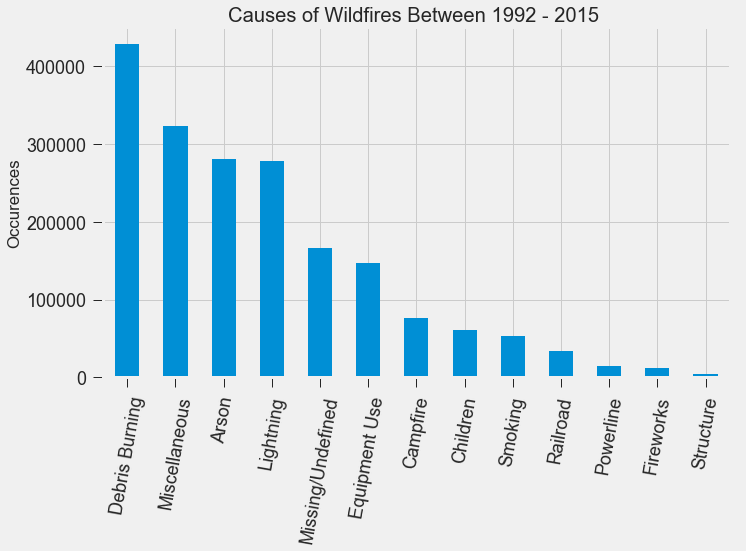 The above graph shows the distribution of wildfire causes in the 24-year period. We can see that over 700,000 cases of wildfires were attributed to two causes: debris burning and "miscellaneous". Debris burning are fires started by people burning trash, crops or other waste materials, and miscellaneous fires are ones that are started by anything that cannot be grouped in any of the other categories, such as fires started by electrical wiring or from other natural sources other than lightning. You can find the description of each category here. I also want to point out the missing/undefined category which I will write about a little later in this blog post. To tackle this dataset, I started with some exploratory data analysis. Exploratory Data Analysis 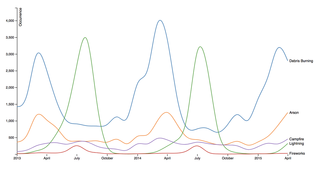 Wildfire Causes Between 2013 - 2015 The plot above highlights five causes of wildfires and plots their total occurrences over time, and by looking at the graph, it's clear that the causes are cyclical. Wildfires caused by debris burning and arson typically happen in late winter or early spring, lightning fires occur in the summer months, and perhaps not surprisingly, wildfires caused by fireworks occur in early July. There also seems to be no apparent pattern for wildfires caused by campfires, which is somewhat surprising. 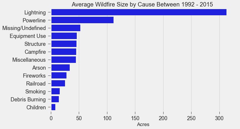 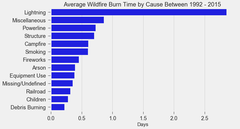 I wanted to explore whether the size of the fire and the number of days it took to contain the fire had any signal on the fire's cause. The above graphs indicates that fires caused by lightning and powerlines result in larger fires compared to fires caused by arson and debris burning, and that lightning-caused fires burns significantly longer other fires. These plots may indicate that wildfires caused by lightning have characteristics that make it easier to distinguish than others. Classification Metrics After trying different combinations of features on different models, the features that seem to have the most signal for the cause of wildfires, listed in order of importance, are as follows:
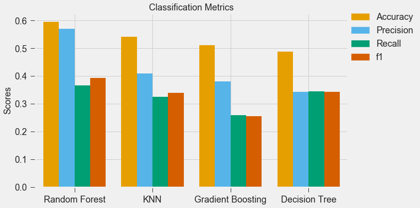 For my classification models, I chose to focus on K-Nearest-Neighbours and tree-based algorithms as these tend to work better with multi-class problems. By using sklearn's GridSearchCV, I tuned my hyper-parameters (k-neighbors, number of trees, tree depth, max features, min sample leafs, etc) and compared the classification metrics to determine the parameters that would yield the highest precision and recall, using macro averages. The graph above shows the results for different models with tuned parameters, where the random forest model seems to have obtained the best accuracy, precision and recall scores. 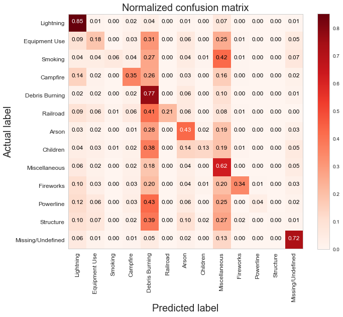 Confusion Matrix - Random Forest Model The above is the confusion matrix for my random forest model normalized to the actual class labels. From the confusion matrix, we can see that my model predicted a lot of false positives for debris burning and miscellaneous. What is interesting is that the accuracy for lightning class is quite high, with 85% of all events predicted correctly, and with much fewer false positives compared to debris burning and miscellaneous cases. This confirms my original hypothesis that lightning caused fires have characteristics that make it more distinguishable than other causes. If we take a look at the predicted versus actual label of the missing/undefined cases, we can also see that the accuracy is quite high, at 72%, with relatively low amount of false positives. This may suggest that wildfires with unknown causes may also share similar characteristics. Prediction of Missing/Undefined Wildfires To further explore these missing/undefined cases, I trained and fit another random forest model without the missing/undefined cases, then I used my trained model to predict on the missing/undefined cases. The graph below shows the predictions of over 70,000 missing/undefined causes of wildfires between 1992 and 2015, and shows that my model predicts almost 30,000 out of the 70,000+ cases of missing/undefined causes of wildfires are caused by arson, based on their location and fire characteristics. 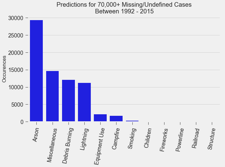 Prediction Application of Wildfire Causes Using this random forest model, I created an interactive Flask application to determine the highest probable cause of a wildfire for a given location, time of the year, days needed to contain the fire, and the size of the fire. I also created a d3 visualization of the total area of fires for a given US state as a proportion of the state's area. I will put links to those once I have it set up. The code for my analysis and visualizations can be found on my GitHub page. 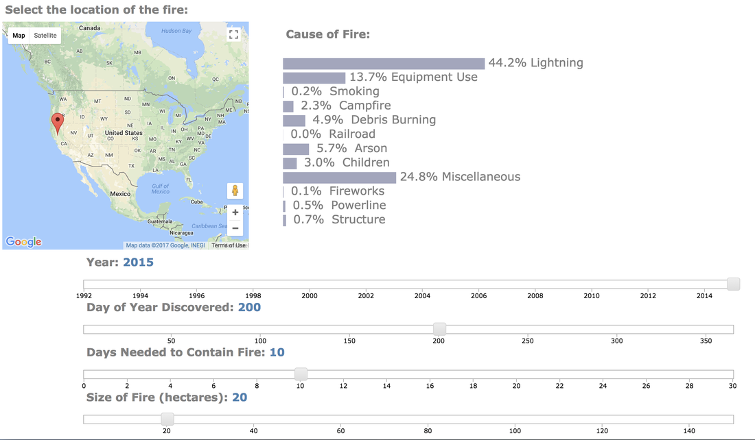 Flask Predictor Application 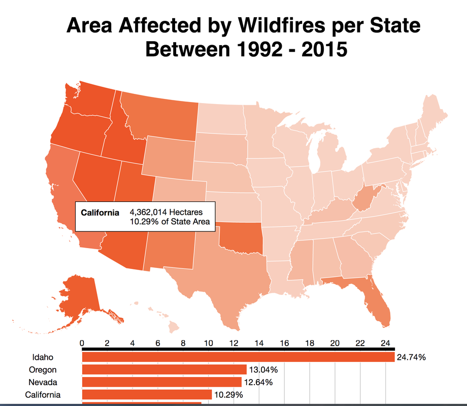 d3 Visualization Conclusions In this post, I've explored some defining characteristics of wildfires and discovered that wildfires caused by lightning may be more easily distinguishable due to its relatively larger size and burn time. I applied a trained random forest model to predict the 70,000+ missing/undefined cases of wildfires over the past 26 years, and the results show that a statistically significant majority of those fires were due to arson. My next blog post will be on my fourth project, codename Fletcher, where the main focus is to use unsupervised machine learning algorithms and natural language processing. The data I plan to use is comments from YouTube videos on the new iPhone X obtained using the YouTube API. By using Python's natural language toolkit (nltk) library, I will process the text data into vectorized data and use clustering algorithms to group the comments, and perform sentiment analysis to summarize each comment cluster to gain insights on how the public feels about certain features of the new iPhone.
0 Comments
It's been almost a month since my last blog post, and I have yet to write about my results from my regression model for Project Luther. We have just finished up with our third project at Metis (codename McNulty), which had a focus on classification models, d3 visualizations, and Flask API and I am eager to talk about it in my next post, but for now I want to show some of my results from Project Luther. This is a continuation of my previous post, so if you have not read it yet, kindly do so before proceeding with this post. Recap To recap on Project Luther, my goal was to create a regression model to predict the effectiveness of an NBA player in their rookie season measured by their box-plus-minus (BPM). I had left off last post with determining colleges that have historically produced drafted NBA players with a higher rookie year BPM, with the restriction that the college needed to have produced more than 5 NBA players. I then ranked these colleges between 1 to 10 and gave players a ranking corresponding to the college they went to if they attended one of these top ten colleges, and 0 otherwise. More Feature Engineering Another feature I wanted to add to my model was how other players on the rookie's NBA team affect the rookie's BPM. To include this feature in my model, I needed to scrape the advanced stats data for all players in the NBA, for each team, and for each season since 2003, which proved challenging given team names change and franchises move cities. My solution for this problem was to first extract a list for all the URL extensions of each team in my time period (for example, /teams/GSW/2017.html for the 2017 Golden State Warriors). Once a had this list, I looped through my URL list to scrape the data I needed, again using BeautifulSoup. The features I created from this data was the Top 3, Top 5, Top 7 and Top 13 players' BPM for each team and each season, and I merged this data to correspond with the team and season a rookie played in. 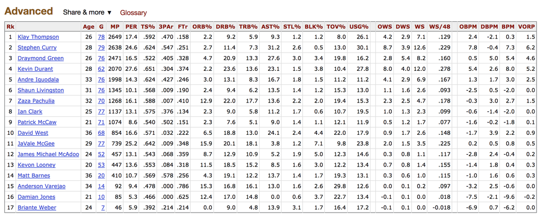 Advanced Stats for 2017 Golden State Warriors Regression Models Now that I have all the data and features I needed, including the college stats I scraped previously, I started training different regression models, using cross-validation methods and tuning parameters using sklearn's GridSearchCV. After trying linear regression models (Lasso and Ridge) and tree based models (random forest and gradient boosting), the best result I got in terms of R-squared was a multiple linear regression model with no regularization with an R-squared of 0.168. 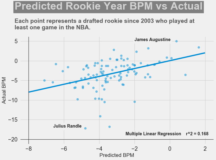 Conclusions I had gone into this project fully understanding that predicting an NBA player's effectiveness in their rookie season was a tough ask, but these results were frankly disappointing. I believe that one of the reasons why the model produced such poor results was the lack of data. Using an 80-20 train-test-split, my holdout set only had about 100 data points. Another reason, in my opinion, why the model did not have much predictive power is that a catch-all per-100-possession statistic like BPM is skewed for players who did not play many possession in their rookie season. Take the graph above, for example. Julius Randle played 14 minutes in 1 game and had a BPM of -16.8 in his rookie season while James Augustine played 7 minutes in 2 games and had a BPM of 5.0 in his rookie season. 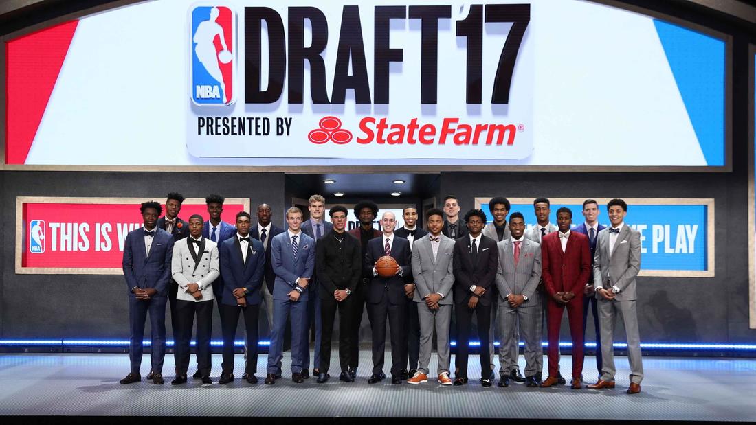 NBA Draft 2017 So how can NBA general managers pick more Blake Griffins (38mpg 22.5ppg 12.1rpg 3.2bpm in his rookie season) and Kevin Durants (34.6mpg 20.3ppg 4.4rpg -1.4bpm in his rookie season), and fewer Kwame Browns and Anthony Bennetts? Well, I suppose if I had a simple answer to that question, I would be getting a lot of NBA teams leaving messages on my phone. Perhaps some other features I could have added to my model were a player's college star rating from recruiters. Another technique I can incorporate into this model is to determine a college player's "hype" from Twitter or basketball forums using natural language processing. Both of these features could perhaps give a better picture of a player's athleticism and potential. These are things I look to add to improve my model, but for the time being, the code for this project can be found on my GitHub.
In my next post, I will be going through my third project, a classification model to predict a cause of a wildfire in the US. |
Kenny LeungPassionate sports fan, wannabe golfer, avid gamer and world traveller. Archives
December 2017
Categories |
 RSS Feed
