|
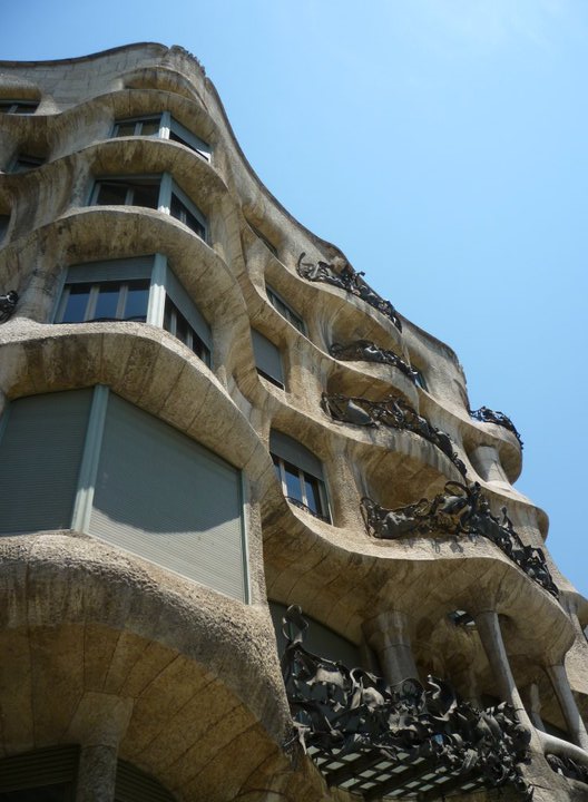
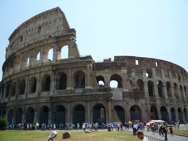
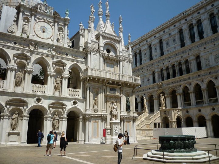
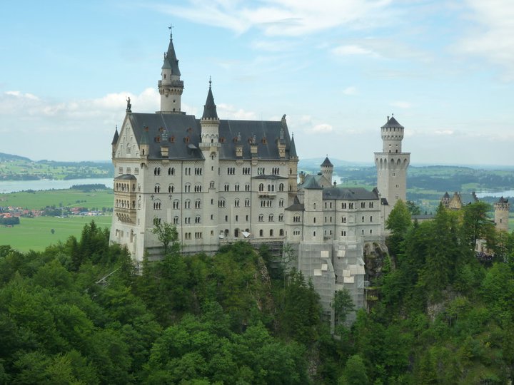
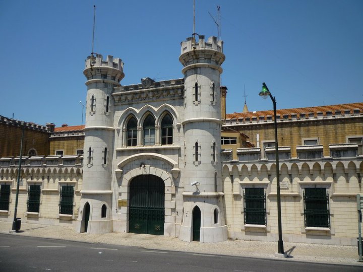
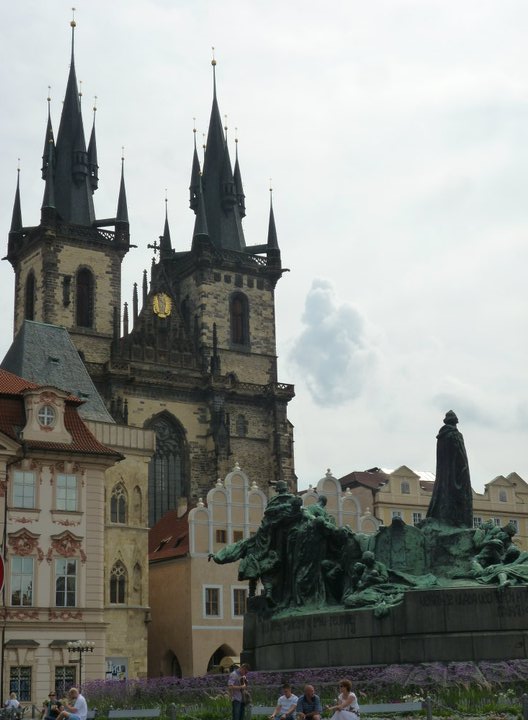
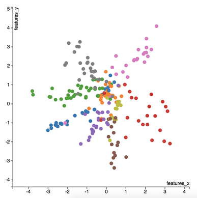
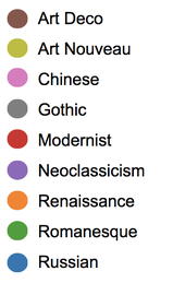
I love to travel. After graduating from university in 2010, I went on a two-month backpacking trip through Europe where I visited 10 different countries and took well over a thousand photos. Aside from trying new foods or learning about the history, one of my favourite things to do during my trip was to take pictures of all of the amazing buildings I came across (here are just a few of the pictures I took during that trip). For architecture enthusiasts, determining a building's architectural style comes down to pattern recognition, and being able to discern shapes and characteristics of a building. If the building has eccentric/irregular forms or sweeping curves (like Casa Milà above), chances are the style is Art Nouveau. Or maybe the building has many arched windows and tall spires (like the Church of Our Lady before Týn), then the building is likely to be Gothic style architecture. For this project, I wanted to explore whether a machine can be trained to recognize these patterns by applying a deep convolutional neural network (CNN) to classify a building's architectural style based on images. Furthermore, to better understand how the trained neural network perceives similarities of building based on images, I wanted to explore two different dimension reduction techniques: variational autoencoders and t-stochastic neighbour embedding (t-SNE). Both of these techniques find faithful representations of high dimensional inputs (like image data) and transforms them into lower dimensions allowing us to more easily make spatial comparisons between images. In this blog post, I will go over my process of using transfer learning to solve my classification problem by fine-tuning a deep learning model in Keras, as well as using Keras and scikit-learn to train a variational autoencoder and to apply t-SNE. Problem Overview Architectural styles often build on one another, with each past period providing inspiration for the next culture. For this project, I decided to choose architectural styles for my target variables that are more distinct and with less overlap in the historical timeline. To this end, I chose 9 different architectural styles to focus my analysis on: Chinese, Romanesque, Gothic, Renaissance, Russian, Neoclassicism, Art Nouveau, Art Deco, and Modernist. Transfer Learning The idea of transfer learning is using pre-trained image models (such as VGG16, VGG19, or InceptionV3) and retraining them on a distinct image classification task. I used the pre-trained InceptionV3 model for this project, and Keras documentation explains step-by-step how we can fine-tune this model to solve our classification problem. 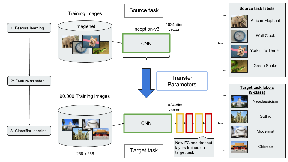 Transfer Learning on InceptionV3 model InceptionV3 is a model trained by Google to classify an image across 1000 categories supplied by the ImageNet academic competition, and has an error rate that approached human performance with a top-5 error rate (how often the model fails to predict the correct answer as one of their top 5 guesses) of 3.46%. Since the early layers of InceptionV3 has captured universal features like curves and edges and are still applicable to other problems with natural images, we want to protect these lower-level features during the back-propagation pass by freezing the weights of the bottom layers of our neural network from updating. Next, I truncated the original softmax layer and replace it with my own classification layer to solve my nine class classification problem, and added two dropout layers prior to this classification layer. Dropout is a regularization technique where randomly selected neurons are ignored during training (the process is explained in this post) to reduce overfitting in neural networks. The below code shows the final architecture of my convolutional neural network. 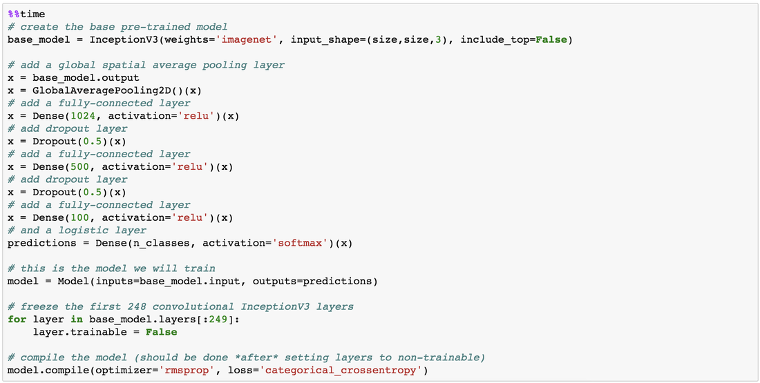 Convolutional Neural Network Architecture Getting Data One advantage of using transfer learning is that you don't need as much data as you would need if you were to train a convolutional neural network from scratch since Google has already done most of the hard work. Another technique we could use to reduce the number of sample images we would need to train our CNN is use image augmentation to increase our number of training samples. To get my training images, I downloaded the images from Google search results of my nine architectural styles using a Firefox add-on called Google Images Downloader. The search results needed to be manually curated to ensure that the image was in fact the correct architectural style as the search parameter, and also to remove any borders or text that may also appear in the image. The search result produced approximately 300 unique photos for each of my target classes (around 2700 images in total). Once I was confident that the sample images were ready to be applied to train my neural network, I first set aside 100 images per target class to be used as a holdout set on my trained model before I processed the rest of my images to be used as a training set. The image processing procedure consists of downsampling my input images to reduce my image size to 256 x 256 pixels. Downsampling input images is a common practice to ensure the model and the corresponding training samples (from a single mini-batch) can fit into the memory of the GPU. I then created synthetic training samples by blurring the input images and applying random translations and rotations. Training on this augmented dataset makes the resulting model more robust and less prone to overfitting. The resulting dataset consisted of 10,000 training samples for each target class, or 90,000 total training images. Setting Callbacks and Model Fitting Callbacks are a set of functions within Keras that allows you to view each state of the model during the training process. For my use case, I was particularly interested in using ModelCheckpoint to save the weights of my model after each epoch, and also EarlyStopping which allows the model to stop training when a monitored quantity (such as validation loss) has stopped improving. A list of callback functions and how to implement them in Keras can be found in the Keras documentation here. 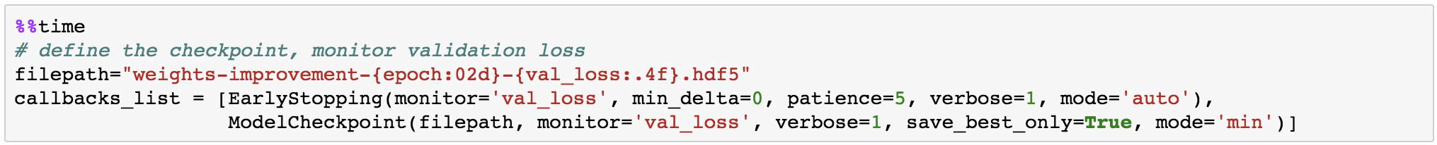 Keras Callback Functions Once my callback functions have been defined, I'm ready to fit the model. The documentation for the Keras fit method and the list of parameters that can be tuned can be found here. By setting an early stopping argument, I can safely set a large number epochs to train the model since I can be confident that once my validation loss has stopped improving, the model will stop training and the weights for the best validation score will be saved. The next parameter that can be tuned is batch_size, which defines the number of samples that will be propagated through the network per gradient update with a default value of 32. A lower batch size has the advantage of requiring less memory and the network typically converges faster as the number of gradient updates is considerable higher than batch gradient descent. A validation set can be held aside to be evaluated on after each epoch by setting the validation_split parameter with a number between 0 and 1, which represents the fraction of the training set to be used as the validation set.  Keras fit Method Classification Metrics After testing different dropout values as well as batch sizes, the values that resulted in the best validation score were: dropout = 0.5, batch_size = 32. I set the patience = 10 (number of epochs with no improvement after which training will be stopped) to be confident that my validation loss has reach a minimum. The below plot shows the bias-variance tradeoff in action, and we can see that after 6 epochs the model is starting to overfit (validation error increases dramatically). 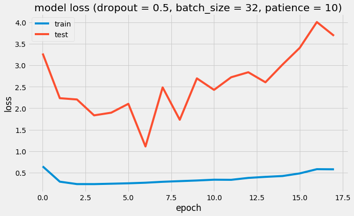 Training and Test Error The resulting model was able to achieve a top-1 error rate of 19.11% and a top-3 error rate of 4.89% when predicting on the holdout set, and below is a confusion matrix for that data. As a reminder, my holdout set consists of 100 samples of each target class, and the images are set aside prior to image augmentation. From the confusion matrix, we can see that Chinese architecture is quite distinct from the other classes, being accurately predicted 97% of the time. The model has the most trouble classifying Renaissance architecture, being accurately predicted only 60% of the time. From the confusion matrix we can see that the model falsely predicts Renaissance as Neoclassical 19 times. Based on the results, we can also see that Renaissance buildings share similar characteristics as Gothic and Romanesque architecture as they are most commonly misclassified. 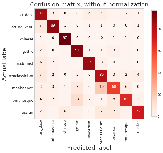 Data Visualization How can we measure similarities between two images? A convolutional neural network looks at an input image through windows in order to find the most important features for classification. For example, a CNN's bottom layers can learn to recognize lines or curves, while its top layers can learn to recognize arches or spires. By truncating the classification, fully-connected, and dropout layers, an input image can be fed into my trained CNN and the output would be a high-dimensional vector of features (in my CNN architecture, the output would be a 1024-dimensional vector). The relative similarity of images can then be calculated based on either cosine similarity or Euclidean distance of these vectors. What if we want to visualize the relative similarities of all the images in our dataset? Unfortunately, human imagination is fairly poor beyond three dimensional data. We need to find ways to reduce our 1024-dimensional data into lower dimensional features and project them into a latent space so that we can visualize them. I will talk about two ways to achieve this: by training a variational autoencoder to learn representations of the input data in lower dimensional space, and by applying t-stochastic neighbour embedding (t-SNE) which maps high dimensional space to a 2D or 3D space. Variational Autoencoder Variational autoencoders (VAE) are a class of unsupervised machine learning models used to generate data, like Generative Adversarial Nets (GAN), and is rooted in bayesian inference in that it learns a latent variable model (parameters of a probability distribution) for its input data and then samples from this probability distribution to generate new data points. There are two main components of an autoencoder: an encoder that compresses high dimensional input data to a bottleneck layer (which is a lower dimensional representation of the input), and a decoder that takes the encoded input and maps these latent space points back to the original input data. The latent space is the space in which the data lies in the bottleneck layer. 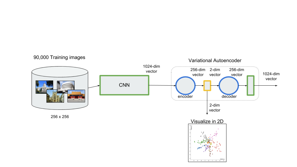 Variational Autoencoder Two practical applications of autoencoders are data denoising, and dimensionality reduction for data visualization. Documentation on how to build autoencoders in Keras can be found here. Using the same 90,000 image training set and 100 image test set I used to train my CNN, I fed these images into the trained CNN with truncated top layers to get 1024-dimensional feature vectors of the training and test images, before applying a MinMaxScaler and using the output to train my variational autoencoder. Once trained, the encoder is able to take any input image and transform it into a 2D representation in the latent space. To understand how my convolutional neural network perceives similarities in images, I took a sample of 223 "famous" buildings around the world where each of my nine architectural styles are represented. The list of buildings, labels, and the image URLs can be found here. I took the representations learned in the latent space and plotted these 2D points in the plot below. The nine different colours represents the nine different architectural styles, and without knowing any of the labels, the variational autoencoder has done a pretty good job clustering these images based on architectural styles.
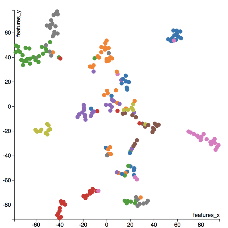
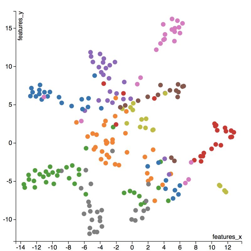
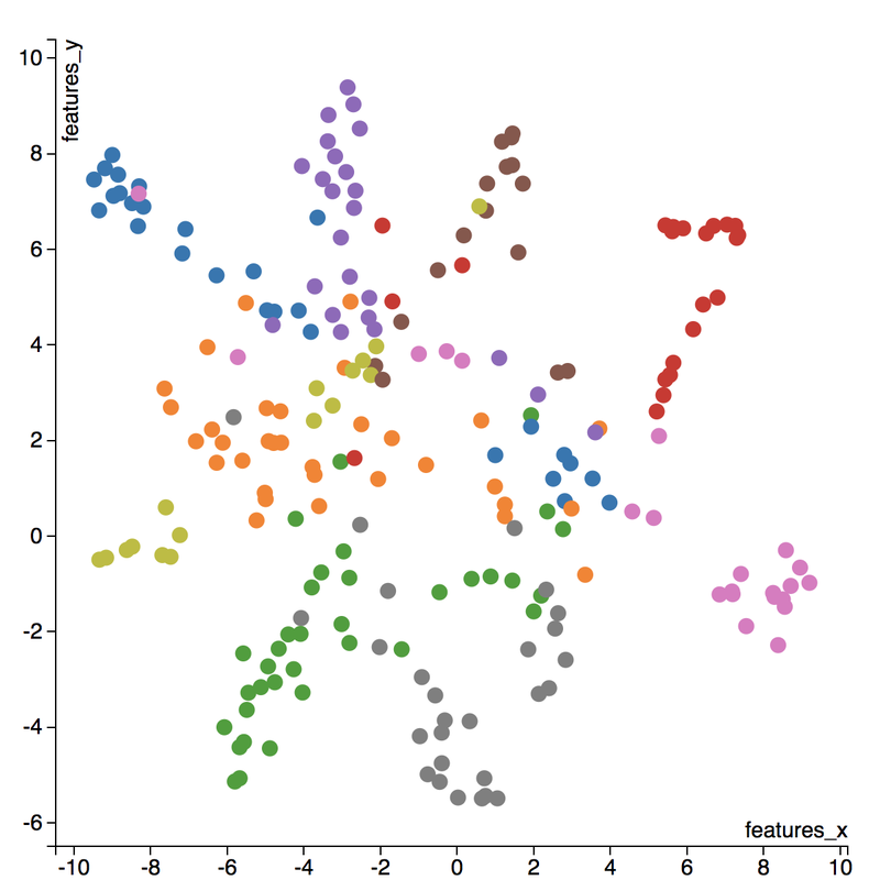
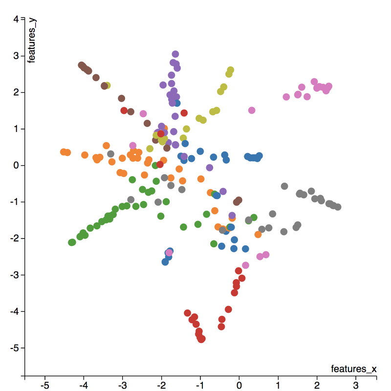
A few insights can be drawn from this plot. Firstly, there is a clear radial shape to the distribution of images, with each spoke representing an architectural style. What is interesting is how the images of Renaissance buildings, represented by the orange dots, are centred at the hub of the radial shape. This result is aligned with the results from the confusion matrix above, where we saw that the Renaissance labeled buildings seem to be the most difficult to classify. We can also see that Renaissance, Gothic, and Romanesque images are relatively close to each other in the latent space, which is a result that was also shown by analyzing the confusion matrix. The pink spoke representing Chinese buildings has a greater angular distance than the other classes, which may suggest some defining characteristics that differ Chinese buildings from other buildings. An educated guess would be that the neural network has learned that sweeping roofs, often characterized in Chinese architecture, is an important feature for classification. Another interesting thing to point out is if you look at the Modernist buildings represented by the red dots, you can see that even though they are clustered together, they are more spread out compared to the other classes, which may suggest that even though those buildings share similar characteristics, such as clean lines or sleek minimalistic styles, they are still very different looking from each other. The video below is visualization I created using d3.js that shows the image of the building that the point represents by hovering over it. By looking at nearby points, it allows us to make spatial comparisons between the images. 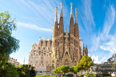 Sagrada Familia Sagrada Familia The video below shows a demonstration of a predictor application I created using Flask and d3.js. Let's say we want to know the architectural style of the Sagrada Familia (pictured on the right) in Barcelona. In the demonstration, I have inputed the image URL in the input field. The application will make a prediction from the convolutional neural network model of the building's architectural style. In this case the model has predicted that the Sagrada Familia is Gothic style architecture. It then finds a 2D representation of the input image using the trained variational autoencoder and plots a point at that location in the latent space, allowing us to look at the dots that are nearby to see which buildings share similar features. t-distributed Stochastic Neighbour Embedding t-distributed stochastic neighbour embedding (t-SNE) is a machine learning algorithm for dimensionality reduction that is particularly well-suited for mapping a high dimensional space to a 2D or 3D space. Imagine our images are plotted in a 1024-dimensional feature space. The algorithm looks at the original dataset that is entered and looks at how to best represent these data points using fewer dimensions, while trying to keep the pairwise distances the same. There are some important differences between t-SNE and variational autoencoders. One main difference is that t-SNE models learn by transductive inference meaning it learns representations from observed, specific training cases to specific test cases. t-SNE is not really applicable beyond the data points it is fed as training. In contrast, variational autoencoders are inductive learners meaning they can learn from observed training cases to general rules, which are then applied to the test cases. This allows for new points to be added to the scatter plot generated by the representations of the input data in the latent space as shown in the video of the predictor application above. Another major difference is that t-SNE typically requires relatively low-dimensional input data. Scikit-learn has an implementation of t-SNE and the documentation can be found here. The documentation highly recommends that another dimensionality reduction method be used to reduce the number of dimensions to 50 if the number of features is very high in order to suppress some noise and speed up the computation of pairwise distances between samples. Using principal component analysis (PCA), I reduced the 1024-dimensional feature vectors of my 223 "famous" buildings to 50 dimensions prior to applying t-SNE. 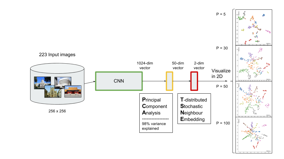 t-distributed Stochastic Neighbour Embedding (t-SNE) A feature of t-SNE is a tuneable parameter, perplexity, which (loosely) translates to how the algorithm balances between local and global aspects of the data. Perplexity can be thought of as a guess about the number of close neighbours each point in your data has. The perplexity value typical ranges between 5 and 50, and has a very complex effect on the resulting plots as shown below. More information on how to tune the parameters and how to interpret t-SNE plots can be found here. Two important takeaways from the linked post is that cluster sizes in a t-SNE plot have very little meaning, and measuring the distances or angles between points in these plots do not allow us to deduce anything specific and quantitative about the data. It is difficult to draw any concrete conclusions from the t-SNE plots with different perplexities, but we can see that the clusters that are generated do split up the images fairly well based on their architectural style. The clusters are also quite similar to those generated by the variational autoencoder with an apparent radial shape at higher perplexities. Conclusions Neural networks are great tools for pattern recognition and image classification, but often times they are considered "black boxes" in that the results can be difficult to interpret. The two dimension reduction techniques I have discussed in this post are excellent ways to visualize the important features that a convolutional neural network uses to perform their classifications. A next step for this project would be to increase the number of target classes and train the CNN and VAE with more images. It would be interesting to explore how the VAE will find representations in 2D space when there are much more target classes. I've also touched on how to create compelling 2D mappings from high-dimensional data using t-SNE. A strength of t-SNE is being able to find structure where other dimensionality-reduction algorithms cannot, but a good intuition on how t-SNE works is needed in order to avoid misinterpretation of the plots. To view the code for this project, please refer to my GitHub page.
3 Comments
luiz
9/13/2018 07:18:19 am
Could you provide the 2700 image data set? The one downloaded from google images and curated. Leave a Reply. |
Kenny LeungPassionate sports fan, wannabe golfer, avid gamer and world traveller. Archives
December 2017
Categories |
 RSS Feed
